In this blog post I will describe the implementation of a first neural network prototype that I developed for my GSoC project. After a presentation of the forward and backward propagation algorithms for the training and evaluation of neural networks in my previous blog post, a first stand-alone neural network prototype has been developed that illustrates the general design for a multi-architecture implementation of neural networks and is used to verify the formulation of the fundamental algorithms that was developed in the previous post.

General Design

The aim of this project is to extend the current implementation of deep neural network in TMVA with functionality for GPU-accelrated training of deep neural networks. This will be achieved by introducing a low-level interface that separates the general algorithms for the training and evaluation of the neural network from the hardware-specific implementations of the underlying numerical operations. On top of the low-level interface sits a generic, object-oriented neural network model that coordinates the training and evaluation of the network. The low-level interface will be implemented by hardware-specific matrix data types that provide the functions required by the interace. The general structure of the implementation is illustrated in the diagram below.

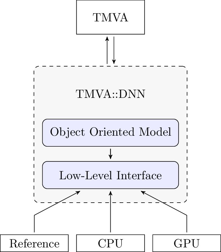
Figure 1: Structure of the neural network implementation.

The Low-Level Interface

In my previous blog post I presented a formulation of the forward and backward propagation algorithms in term of matrix operations. Based on this we can now identify the fundamental numerical operations that are required for the foward and backward propagation in oder to define the low-level interface. Note that the description of the low-level interface given below is only a very brief outline of the actual interface. The complete specification can be found here.

Forward Propagation

The fundamental operations required to compute the neuron activations \(\mathbf{u}^l\) of a given layer \(l\) from the activations of the previous layer \(l-1\) are the following:

• Computation of the matrix product \(\mathbf{U}^{l-1} (\mathbf{W}^l)^T\) of the matrix activations of the previous layer and the weight matrix of the current layer
• Row-wise addition of the bias vector \(\boldsymbol{\theta}^l\)
• Application of the activation function \(f^l\) to each element of the resulting matrix

In addition to that, we also need to evaluate the first derivatives of the activation function \(f^l\) at \(\mathbf{U}^{l-1}(\mathbf{W}^l)^T + \boldsymbol{\theta}^l\), which are required in the backpropagation step.

Backward Propagation

In a single step of the backpropagation algorithm the gradients of the loss function of the network with respect to the weights and bias variables of the current layer as well as the activations of the previous layer are computed. Since the computations involved here produce common intermediate results that can be reused during computation , we do not split up the computation but require the low-level implementation to provide a function that implements a complete backpropagation step for a given layer.

Additional Operations

In addition to the fundamental operations for forward and backward propagation, the training and evaluation of a neural network require further operations on the weight and activation matrices of each layer:

• Loss function: Evaluation and computation of the gradients of the loss function of the network.
• Output function: Computation of the nerual network prediction from the activations \(\mathbf{U}^{n_h}\) of the last layer in the network.
• Regularization: Evaluation of the contribution of regularization terms to the loss of the network and their contribution to the gradients of loss function with respect of the weights of each layer.
• Addition and Scaling: For the updating of the weight matrices during training of the network it is necessary to add and scalte weight and gradient matrices.

The Neural Network Prototype

Based on the low-level interface outlined above, a first neural network prototype consisting of a reference implementation of the low-level interface and a first object oriented neural network model has been developed.

Implementation Model

The current implementation model consists of two main class templates, a Net class template and a Layer class template. The Net class defines the network structure of the neural network through a vector of Layer objects. The layer class handles all the memory that is required during the execution of the forward and backward propagation steps. All class templates in the implementation take as type argument an Architecture type parameter that holds the data types used for the representation of scalars and matrices for a specific architecture. In addition to that, the Net class takes a LayerType type parameter that specifies the type of the layer used in the net. This is required to handle nets that hold their own weight matrices as well as nets that use the weights of another network. The general class structure of the object-oriented neural network model of the first prototype is given in the figure below.

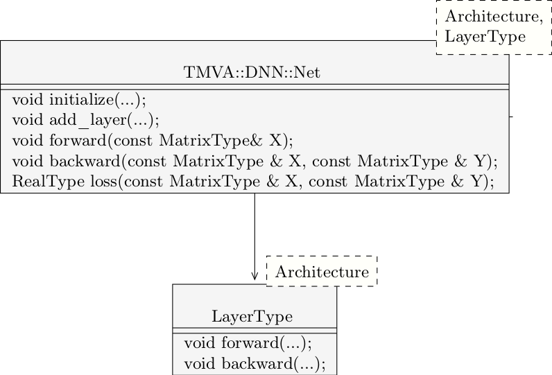
Figure 2: Class structure of the first neural network prototype.

The Reference Architecture

The reference architecture developed for the prototype uses ROOT’s TMatrixT generic matrix type to implement the low-level interface. Its purpose is of course only the verification of the neural network prototype and to serve as a reference for the development of optimized, architecture-dependent implementations of the low-level interface. The Architecture type template representing the reference architecture is given below.

template<typename Real>
struct Reference
{
public:
    using RealType   = Real;
    using MatrixType = TMatrixT<Real>;
};

The complete implementation of the neural network prototype is available on github in my fork of the ROOT repository.

Testing

Since the formulation of the foward and backward propagation algorithms is quite complex, the implementation was thoroughly tested in order to ensure its correctness. One of the primary tests was the verification of the gradients computed using the backpropagation algorithm. This was done by comparing the gradients computed using backpropagation with gradients computed using numerical differentiation. Since this test covers both the forward and backward propagation through the network, it should make us quite confident about the correctness of the implementation if passed by the prototype.

For each such network, the maximum relative error in the gradients has been computed. One constraint here was that the activation functions of the neural network must be differentiable and therefore only linear and sigmoid activation functions were considered. For all tests presented below the mean squared error loss function was used.

Slight problems were encountered here since the division by the width \(2\Delta x\) of the difference interval leads to loss of precision. In order to investigate this, an additional test was performed using only the identity function as activation functions. Since the resulting neural network is a linear function of the input matrix, the loss function is quadratic and the central difference quotient is exact for all interval widths \(2\Delta x\). That means that the gradients in this case can be computed without the loss of precision resulting from the division by the width of the difference interval by choosing \(2\Delta x\) to be the unit close to \(1\). The maximum relative errors of the weight gradients with respect to the half width of the difference interval \(\Delta x\) are displayed in the plot below. As can be seen from the plot, for the linear net the relative error of the gradients lies within the range expected for double precision arithmetic. Also clearly visible is the increase in error with the depth of the network.

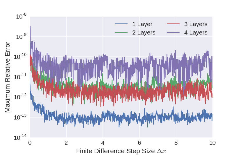
Figure 3:Maximum relative error of the weight gradients computed using backpropagation and numerical derivation for a linear neural network.

The testing results for a non-linear net with sigmoid activation functions is displayed in Figure 4 below. For a non-linear net, the finite difference interval used for the computation of the numerical error must be reduced in order to obtain a good approximation to the derivatives. However, the required division by the interval width amplifies the numerical error in the results and thus leads to a loss of precision. This can be clearly seen in the plot below, which displays the maximum relative error of the weight gradients with respect to the half width \(\Delta x\) of the finite difference interval for increasing depths of the neural network. One can clearly identify two different error regimes in the plot: For finite difference intervals greater than \(\sim 10^{-4}\), the maximum relative error decreases with the interval width. In this region the approximation error of the difference quotient used for the numerical computation of the gradients is dominates the numerical error due to finite precision arithmetic. For \(\Delta x < 10^{-4}\), the error increases again which is due to numerical error that is amplified due to the division by the interval width. This claim is supported by the behaviout of the numerical error for the linear net, which are displayed in the background of the plot.

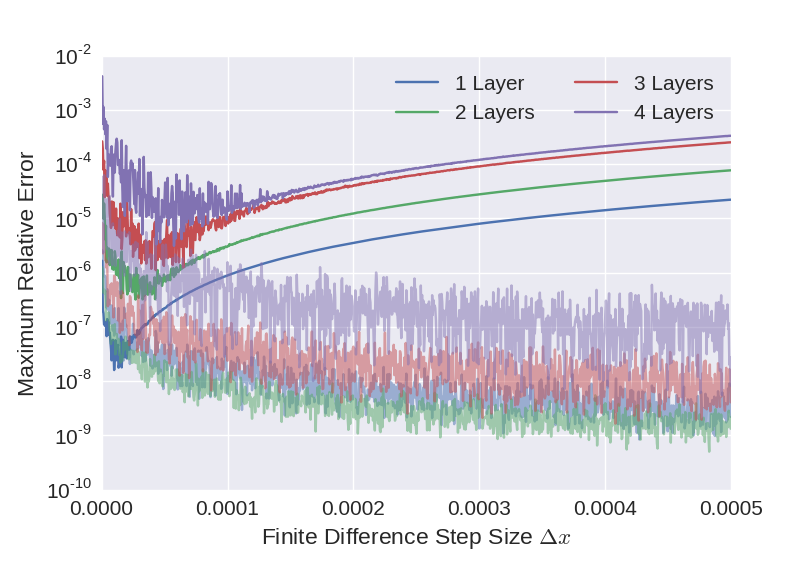
Figure 4: Maximum relative error of the weight gradients computed using backpropagation and numerical derivation for a non-linear neural network using Sigmoid activation functions. The curves in the background displayed the numerical error for the corresponding linear net.

Summary and Outlook

In this blog post a first stand-alone prototype of a multi-architecture implementation of deep neural networks was presented and the implementations of forward and backward propagation verified by comparison of the computed gradients with numerically computed gradients. The next step is now the integration of the prototype into TMVA and to perform a first end-to-end test by training the network on the Higgs data set.