Deep Neural Networks and the Backpropagation Algorithm
Two weeks have now passed since the beginning of the coding phase of the 2016 Google Summer of Code. In this blog post, I will present the main results of the first week working on my project GPU-accelerated deep neural networks in TMVA. The starting point of my project is a prototypical implementation of deep neural networks in TMVA, which is included in the latest ROOT version. The aim of my GSoC project is to extend this implementation so that neural networks can be trained more efficiently, in particular to realize GPU-accelerated training of deep neural networks.
For the kick-off week of the project, I traveled to CERN to meet my supervisors Sergei V. Gleyzer and Lorenzo Moneta and the other members of the CERN SFT group. This was a great opportunity to discuss the project in detail as well getting opinions on the implementation from other ROOT developers.
The first week was then mainly spent getting to know the current deep neural network implementation in depth and writing a detailed project plan that introduces a low-level interface for the offloading of the training to accelerator architectures. The main result of the first week is a detailed description of the neural network model and the operations involved in the training process, which will form the foundation for the implementation of accelerated deep neural networks.
The Neural Network Model
For now, this implementation of neural networks is restricted to feed forward neural networks. In particular, we assume that the activations \(\mathbf{u}^l\) of layer \(l\) are given in terms of the activations of the previous layer by
\[ \mathbf{u}^l = f^l \left ( \mathbf{W}^l\mathbf{u}^{l-1} + \boldsymbol{\theta}^l \right ) \]
for a given weight matrix \(\mathbf{W}^l\), bias terms \(\boldsymbol{\theta}^l\) and activation function \(f^l\) of the current layer. For the training of neural networks, a loss function \(J(\mathbf{y},\mathbf{u}^{n_h})\) is specified, which is minimized using gradient-based minimization techniques. The loss function \(J\) quantifies the error of a neural network prediction \(\mathbf{u}^{n_h}\), i.e. the activations of the output layer, with respect to the truth \(\mathbf{y}\). In addition to that the loss function may also include regularization contributions from the parameters of the network. During training of the network, the gradients of \(J\) with respect to the weights \(\mathbf{W}^l\) and bias terms \(\mathbf{\theta}^l\) of each layer are computed using the backpropagation algorithm. The forward and backward propagation of the training data through the neural network are the performance-critical operations which have to be performed during each iteration of the training of the neural network. In general, the computation of the gradients of the layer is performed using only a small fraction of the training data, a so called mini-batch of a given batch size. Both, the propagation of the neuron activations forward through the network as well as the backward propagation of the error through the network are inherently parallel. By considering the propagation of the training data from a full mini-batch through the network, it is possible to formulate the forward and backward propagation solely in terms of matrix operations, that can be performed very efficiently on massively parallel accelerator architectures. To this end, consider the training data of a mini-batch given by a two-dimensional tensor \(x_{i,j}\) . For ease of notation, simplified Einstein notation will be used in the following, meaning that repeated indices on the right-hand side of an equation imply summation over those indices, if they don’t appear on the left-hand side of the equation. The forward propagation of the activations corresponding to the input batch \(x_{i,j}\) and the backward propagation of the corresponding gradients are described described in the following two sections.
Forward Propagation
Since we are considering the propagation of the complete mini-batch through the neural network, the activations of a given layer \(l\) can be represented by a two dimensional tensors \(u^l_{i,j}\), with the first index running over the neurons of the given layer and the second index running over the features of each sample. The activations of layer \(l\) are then just given by
\[ u^l_{i,j} = f^l\left ( W_{j,k} u^{l-1}_{i,k} + \theta_j \right ) \]
For the forward propagation of the neuron activations, we thus need to compute the tensor product \(W_{j,k}u^{l-1}_{i,k}\), which can be implemented as a straight-forward matrix-matrix multiplication \(\mathbf{U}^{l-1}\mathbf{W}^T\). In the next step, the bias vectors \((\boldsymbol{\theta})_j=\theta_j\) must be added row-wise to the result of the matrix product. Finally, the activation function \(f^l\) of the layer must be applied element-wise to the resulting matrix. The involved computations are illustrated in the figure below.
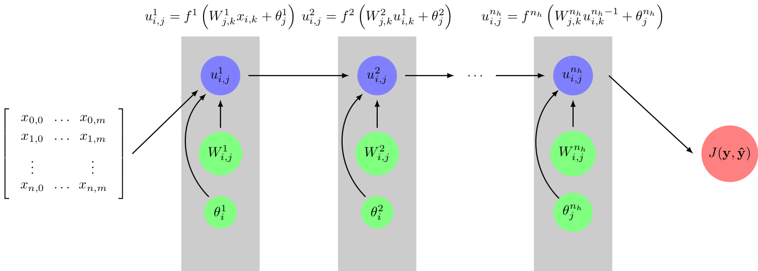
Figure 1: Forward propagation of the neuron activation through the neural network.
Propagating the input mini-batch \(x_{i,j}\) forward through the neural network, yields the corresponding predictions of the neural network. Here we assume the output of the network to be given by the activations of the last hidden layer \(l_{n_h}\) of the network. Depending on the task, these outputs may have to be transformed into a probability or a class prediction. For the training only the value of the loss function corresponding to the activations \(u_{i,j}^{l_h}\) of the output layer and the true output \(y_{i,j}\) is required.
Backward Propagation
The aim of the neural network training is to find weights \(W_{i,j}^l\) and bias values \(\theta^l_j\) that minimize the cost function \(J(\mathbf{y}, \mathbf{u}^{l_h})\). To this end, we need to compute the gradients of \(J\) with respect to the weights \(W^l_{i,j}\) and bias terms \(\theta^l_j\) of each layer. Formulas for the recursive computation of these gradients can be found by repeated application of the chain rule of calculus to the formulas for forward propagation given above:
\[ \begin{aligned} \frac{dJ}{dW^l_{i,j}} &= u^{l-1}_{m,j} (f^l)'_{m,i} \frac{dJ}{du^l_{m,i}} + R(W^l_{i,j}) \label{eq:bp1} \\ \frac{dJ}{d\theta^l_{i}} &= (f^l)'_{m,i} \frac{dJ}{du^l_{m,i}} \\ \frac{dJ}{du^{l-1}_{i,j}} &= W^l_{n,j}(f^l)'_{i,n} \frac{dJ}{du^l_{i,n}} \label{eq:bp2} \end{aligned} \]
Here we use \((f^l)'_{i,n}\) to denote the first derivatives of the activation function of the layer \(l\) evaluated at \(t_{i,j} = W^l_{j,k}u_{i,k} + \theta_j\). The term \(R(W_{i,j}^l)\) is used to represent potential contributions from regularization.
To start the backpropagation the partial derivatives of the cost function \(J\) with respect to the activations \(u_{i,j}^{n_h}\) of the output layer are required. Then for each layer the following operations have to be performed:
Compute the weight gradients \(\frac{dJ}{dW^l_{i,j}}\): Multiply the matrix \((u^{l-1}_{i,j})^T\) with the element-wise product of the derivatives \((f^l)'_{i,j}\) of the activation function and the gradient of the loss function \(\frac{dJ}{du^{l}_{i,j}}\) with respect to the activations of the current layer.
Compute the bias gradients \(\frac{dJ}{d\theta^l_{j}}\): Sum over the columns of the element-wise product of the derivatives \((f^l)'_{i,j}\) of the activation function and the gradient of the loss function \(\frac{dJ}{du^{l}_{i,j}}\) with respect to the activations of the current layer.
Compute the activation gradients \(\frac{dJ}{du^{l-1}_{i,j}}\) of the previous layer: Multiply the element-wise product of the derivatives \((f^l)'_{i,j}\) of the activation function and the gradient of the loss function \(\frac{dJ}{du^{l}_{i,j}}\) with respect to the activations of the current layer with the weight matrix \(W^l_{i,j}\).
The computations are illustrated once more in the figure below:
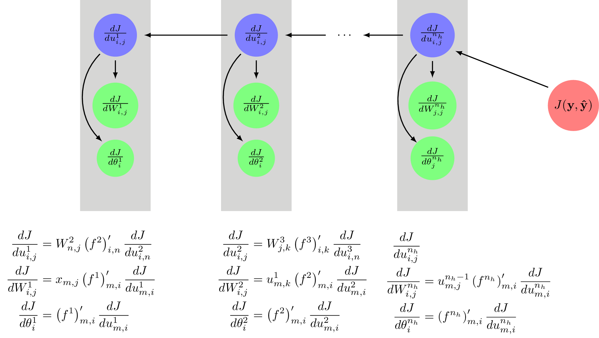
Figure 2: Backward propagation of the error of the neural network predicting through the neural network.
Summary and Outlook
Above we have identified the mathematical structures and operations that are required for the training of neural networks. Moreover we have formulated the forward and backward propagation steps involved in the training of neural networks in terms of matrix operations, which can be very efficiently implemented on accelerator devices such as GPUs. The next step is now the specification of a low-level interface to separate the compute-intense mathematical operations, which will be performed on the accelerator device, from the coordination of the training, which will be performed on the host. This interface together with a prototype implementation will be described in my next blog post.