Deep Neural Networks in TMVA
In order to get familiar with TMVA and introduce the first benchmark dataset, this post will demonstrate how TMVA can be used to train a deep neural network classifier on the Higgs-Higgs dataset as described in the paper by Baldi, Sadowski and Whiteson.
The Data
The Higgs-Higgs dataset consists of simulated 8 TeV collisions from the LHC experiment. The classification task that we are dealing with here is to decide whether during the observed event an electrically-neutral Higgs boson was observed or not. The events of interest, i.e. where the creation of electrically-neutral Higgs boson was observed, are referred to as the signal, while the remaining, uninteresting events are referred to as the background.
In the signal process \((gg \rightarrow H)\), a heavy, electrically neutral Boson is formed, which decays into a heavy, electrically charged boson \(H^{\pm}\) and a \(W\) Boson. The electrically charged Higgs boson then decays into a second \(W\) boson and a light Higgs boson \(h^0\).
This process is overshadowed by a similar process in which two top quarks are formed, which then each decay to a bottom quark and a W boson. This is the background process.
Getting Started With TMVA
TMVA is integrated into ROOT. The traditional way of using it is thus by writing a ROOT macro, which we will call train_higgs():
#include "TFile.h"
#include "TString.h"

#include "TMVA/Factory.h"
#include "TMVA/Tools.h"
#include "TMVA/DataLoader.h"
#include "TMVA/TMVAGui.h"

void train_higgs( )
{
    TMVA::Tools::Instance();

    TString infilename = "higgs.root";
    TFile *input = TFile::Open(infilename);

    TString outfilename = "TMVA.root";
    TFile *output = TFile::Open(outfilename, "RECREATE");

    TMVA::DataLoader *loader=new TMVA::DataLoader("higgs");
    TMVA::Factory *factory = new TMVA::Factory( "TMVAClassification",
                                                 outputFile,
                                                "AnalysisType=Classification" );
Preparing the Data
The original Higgs-Higgs dataset is provided in .csv format. Since the set is very large we here use the dataset converted into .root format which is available from Omar Zapatas homepage.
First off, we create the data handles for input and output files and instantiate a TMVA::Factory, which will handle the training and evaluation of the network for us. Moreover, we create a DataLoader object which will provide the data to TMVA. The input file contains two trees, one containing the signal and the other containing the background events. We extract the trees, add the variables and the two trees to the DataLoader object.
    TTree *signal     = (TTree*)input->Get("TreeS");
    TTree *background = (TTree*)input->Get("TreeB");

    loader->AddVariable("lepton_pT",'F');
    loader->AddVariable("lepton_eta",'F');
    loader->AddVariable("lepton_phi",'F');
    loader->AddVariable("missing_energy_magnitude",'F');
    loader->AddVariable("missing_energy_phi",'F');
    loader->AddVariable("jet_1_pt",'F');
    loader->AddVariable("jet_1_eta",'F');
    loader->AddVariable("jet_1_phi",'F');
    loader->AddVariable("jet_1_b_tag",'F');
    loader->AddVariable("jet_2_pt",'F');
    loader->AddVariable("jet_2_eta",'F');
    loader->AddVariable("jet_2_phi",'F');
    loader->AddVariable("jet_2_b_tag",'F');
    loader->AddVariable("jet_3_pt",'F');
    loader->AddVariable("jet_3_eta",'F');
    loader->AddVariable("jet_3_phi",'F');
    loader->AddVariable("jet_3_b_tag",'F');
    loader->AddVariable("jet_4_pt",'F');
    loader->AddVariable("jet_4_eta",'F');
    loader->AddVariable("jet_4_phi",'F');
    loader->AddVariable("jet_4_b_tag",'F');
    loader->AddVariable("m_jj",'F');
    loader->AddVariable("m_jjj",'F');
    loader->AddVariable("m_lv",'F');
    loader->AddVariable("m_jlv",'F');
    loader->AddVariable("m_bb",'F');
    loader->AddVariable("m_wbb",'F');
    loader->AddVariable("m_wwbb",'F');

    Double_t signalWeight = 1.0;
    Double_t backgroundWeight = 1.0;
    loader->AddSignalTree    (signal,     signalWeight);
    loader->AddBackgroundTree(background, backgroundWeight);
Finally, we define the size of the training and test sets. Here, we only consider \(10^5\) training events and \(10^4\) test events in order to keep the time required to train the network on a common laptop machine at a reasonable level.
    TString dataString = "nTrain_Signal=100000:"
                         "nTrain_Background=100000:"
                         "nTest_Signal=10000:"
                         "nTest_Background=10000:"
                         "SplitMode=Random:"
                         "NormMode=NumEvents:"
                         "!V";

    loader->PrepareTrainingAndTestTree("", "", dataString);
Defining the Network
The network conifguration is passed to the DNN implementation through the BookMethod function using a configuration string to encode the parameters of the net. Different parameters are seperated by colons :.
We start be setting the general TMVA parameters H and V in order to disable help output (!H) and enable logging of the training process (V):
TString configString = "!H:V";In addition to that, we add a variable transformation, that normalizes all input variables to zero mean and unit variance.
configString += ":VarTransform=N";Cost Funtion
Since we are dealing with a two-class classification, i.e. want to distinguish background events from signal events, the appropriate cost to minimize is the cross entropy over the training set.
configString += ":ErrorStrategy=CROSSETROPY";Weight Initialization
The initial weight values are chosen according to the Xavier Glorot & Yoshua Bengio method
configString += ":WeightInitialization=XAVIERUNIFORM";Network Topology
For the network topology, we choose a network consisting of three hidden layers with 100, 50 and 10 neurons, respectively. As activation function the \(\tanh\) function is used for the hidden layers while the output is left linear, since the logit transformation is performed by the cross entropy cost function. The corresponding configuration string takes the form
TString layoutString = "Layout=TANH|100,TANH|50,TANH|10,LINEAR";Training Strategy
We split the training up into three phases. The first one starts with a learning rate of \(10^{-1}\) and a momentum of \(0.5\). In addition to that we add dropout with a fraction of \(0.5\) for the second and third layer. To prevent overfitting we regularize the weights using L2 regularization multiplied by a weighting factor of \(10^{-3}\). The Repetitions option defines how often how often the net is trained on the same minibatch before switching it. The current performance of the net is evaluated every TestRepetitions steps on the test set. The ConvergenceSteps option defines howmany training steps must be performed without performance improvement before the net is declared to have converged.
    TString trainingString1 = "TrainingStrategy="
                              "LearningRate=1e-1,"
                              "Momentum=0.5,"
                              "Repetitions=1,"
                              "ConvergenceSteps=300,"
                              "BatchSize=20,"
                              "DropConfig=0.0+0.5+0.5+0.0,"  // Dropout
                              "WeightDecay=0.001,"
                              "Regularization=L2,"
                              "TestRepetitions=15,"
                              "Multithreading=True";
For the second training phase, we reduce the learning rate to \(10^{-2}\), set the momemtum to \(0.1\) and reduce the dropout in the second and third layer to 0.1.
    TString trainingString2 = "| LearningRate=1e-2,"
                              "Momentum=0.1,"
                              "Repetitions=1,"
                              "ConvergenceSteps=300,"
                              "BatchSize=20,"
                              "DropConfig=0.0+0.1+0.1+0.0,"  // Dropout
                              "WeightDecay=0.001,"
                              "Regularization=L2,"
                              "TestRepetitions=15,"
                              "Multithreading=True";
For the final training phase, we further reduce the learning rate by a factor of \(10\) and set momentum and dropout probabilites to \(0\). In addition to that we increase the batch size to \(50\).
    TString trainingString3 = "| LearningRate=1e-3"
                              "Momentum=0.0,"
                              "Repetitions=1,"
                              "ConvergenceSteps=300,"
                              "BatchSize=50,"
                              "WeightDecay=0.001,"
                              "Regularization=L2,"
                              "TestRepetitions=15,"
                              "Multithreading=True";
So far, we have defined all necessary network parameters. Now we need to book the corresponding neural networks with the TMVA::Factory object, which will take care of training and evaluation of the neural network classifiers. In order to compare the effects of the different training schemes, we book three neural network classifiers: one executing only the first training phase, one executing the first and the second and another executing all training phases. We name the corresponding classifiers according to the number of training phases DNN 1, DNN 2 and DNN 3.
    configString += ":" + layoutString + ":" + trainingString1;
    factory->BookMethod(loader, TMVA::Types::kDNN, "DNN 1", configString);

    configString += trainingString2;
    factory->BookMethod(loader, TMVA::Types::kDNN, "DNN 2", configString);

    configString += trainingString3;
    factory->BookMethod(loader, TMVA::Types::kDNN, "DNN 3", configString);

    factory->TrainAllMethods();
    factory->TestAllMethods();
    factory->EvaluateAllMethods();

    output->Close();
Results
The above code trains three identical neural networks with the three different training schemes given. The ROC curves of the resulting network are displayed below.
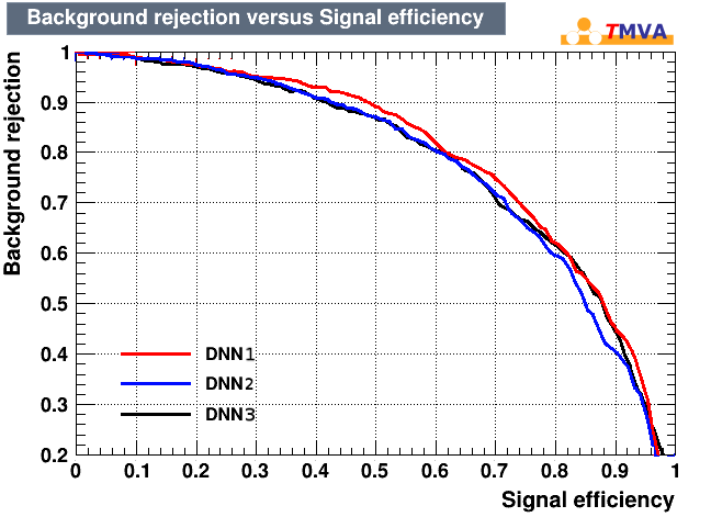
Figure 1: ROC Curves for the three different training schemes. No improvement in classification performance can be achieved through the additional training phases.
Unfortunately no improvement in performance could be achieved from the additional training phases. It even seems that the additional training degrades the classifier performance. This may indicate that the reduction in dropout leads to overfitting of neural network.
One difficulty in training the neural network is that the training currently takes a lot of time. As displayed in the figure below, for the three training phases the times required for the training on my laptop were \(8.1\), \(11.4\) and \(18.8\) hours, respectively. This makes optimizing the network structure and training schemes difficult.
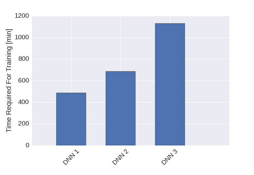
Figure 2: Training times required for the three training schemes described above.