Performance Analysis
The ability to train models efficiently on very large sets of data is a crucial aspect of deep learning techniques. Since the backprop algorithm used for the training of neural networks exposes a high degree of parallelism it can be efficiently implemented on modern, massively parallel accelarator devices such as general pupose graphics processing units. The aim of this project was to make the computational power of those devices accessible to physicists using the Root data anlysis framework. Therfore, a thorough analysis of the performance of the developed code is essential in order to identify performance deficits and finally ensure that deep neural networks can be trained efficiently with this implementation.
Performance Model
Since measuring the execution time alone does not provide much useful information about the efficiency of the code, the following simple performance model is used to assess the performance of the implementation.
The largest part of the time required for the training is spent forward and backward propagating the mini-batches through the network. Consider a layer \(l\) with \(n_l\) neurons, a batch size of \(b_n\). For simplicity weight decay and dropout will be ignored in the following.
Foward Propagation
For the forward propagation through the layer the following operations must be performed:
- Multiplication of the input matrix with the transpose of the weight matrix \(\mathbf{W}^l\) of the current layer.
- Addition of the bias terms to each row of the resulting matrix
- Application of the activation function and evaluation of its derivatives
A common measure for the computational complexity of numerical comupations are the number of floating point oprations (FLOPs) required for their execution. For the matrix multiplication and the addition of the bias terms, these are straight forward to derive. The application of the the activation function is harder to quantify using FLOPs not only because it depends on the function but also because the equivalent number of FLOPs depends on the underlying hardware. However, as will be seen below, their contribution to the overall numerical complexity is low and the application of the activation function will therfore be counted as a single flop. The number of floating point operations for the forward propagation through a given layer is summarized in the table below.
| Operation | FLOPs |
|---|---|
| Matrix Multiplication | \(n_b n_l (2n_{l-1} - 1)\) |
| Addition of Bias Terms | \(n_b n_l\) |
| Activation Function Application | \(n_b n_l\) |
| Activation Function Derivatives | \(n_b n_l\) |
Backward Propagation
For the backward propagation of the gradients through a layer and the computation of the weight and bias gradients the following operations are required:
- Computation of the Hadamard product of the activation gradients with the derivatives of the activation function.
- Multiplication of the resulting matrix with the weight matrix to obtain the activation gradients of the previous layer.
- Multiplication of the hadamard product with the activation to obtain the weight gradients.
- Summation over the columns of the hadamard product matrix to obtain the bias gradients.
The required floating point operation are given in the table below:
| Operation | FLOPs |
|---|---|
| Hadamard Product | \(n_b n_l\) |
| Matrix Multiplication | \(n_l n_{l-1} (2 n_b - 1)\) |
| Summation of Columns | \(n_l (n_b - 1)\) |
Total
Using the formulas in the tables above, the computational throughput in floating point operations per second FLOPS = FLOPs / s for an arbitrary network is given by: \begin{align} \sum_l 6n_l n_b n_{l-1} + 4 n_l n_b - n_l(n_{l-1} + 1) - n_bn_{l-1} \end{align}For hidden layers with a large number of neurons \(n_l\), the above sum will be dominated by the terms involving the triple product \(n_b n_l n_{l-1}\). These terms originate from the matrix products that have to be computed during forward and backward propagation. One can thus expect that matrix multiplication is the critical operation for the performance of the neural network implementation.
The Training Benchmark
Using the formula above, the numerical throughput of the deep neural network implementation has been computed on a benchmark training set. The benchmark training set consists of \(5 \times 10^5\) samples from a random, linear mapping \(f: \mathbb{R}^{20} \to \mathbb{R}\). The network used for the benchmark had 5 hidden layers, each with \(256\) neurons using \(tanh\) activation functions.
CPU Performance
To set a baseline, we begin be examining the performance on a multi-core CPU platform. The benchmarks have been performend on an Intel Xeon E5-2650 with \(8 \times 2\) cores. The CPU backend of the neural network implementation uses multi-threaded BLAS for parallel matrix algebra and TBB to parallelize the remaining operations required for the training. For the benchmarks the OpenBLAS implementation of BLAS was used. The graph below depicts the numerical throughput achieved with respect to the number of threads used for the linear algebra routines. The batch size used was \(n_b = 1024\) samples.
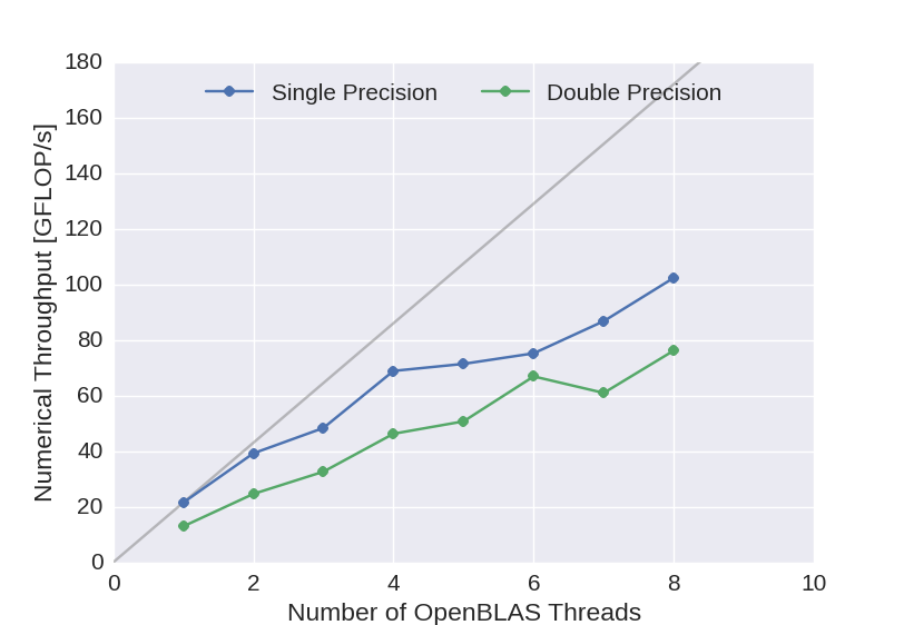
Figure 1: Numerical throughput achieved with the multi-core CPU backend of the newly developed deep neural network implementation.
The gray line indicates ideal scaling of the single-core performance for single precision arithmetic. The performance scales acceptably well with the number of cores used for the matrix arithmetic and overall a numerical throughput of about 100 GFlop/s has been obtained using single precision arithmetic and 80 GFlop/s using double precision arithmetic.
GPU Performance
The benchmarks for the GPU performance have been performed on an Nvidia Tesla K20, which has a single precision peak performance of \(3.52\) TFlop/s and a double precision peak performance of \(1.17\) TFlop/s.
Cuda Backend
The graph below shows the numerical throughput achieved using the CUDA backend of the neural network implementation with respect to the batch size used for the training. In addition to the performance of the benchmark network with \(256\) neurons (blue), also the performance of networks with \(384\) (green) and \(512\) (red) neurons in the hidden layers are displayed. Compared to the theoretical peak performance of the device, the performance is relatively low. This can be improved, however, by increasing the complexity of the network. This indicates that for the not so dense layers, insufficient parallelism is available to fill the GPU.
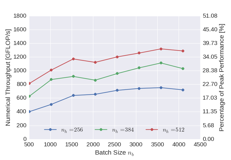
Figure 2: Numerical throughput achieved with the CUDA GPU backend of the newly developed deep neural network implementation using single precision floating point arithmetic.
Multiple Compute Streams
Since the results from the straight-forward implementation indicate that insufficient parallelism is available to keep the GPU busy, we investigated if the performance can be improved by exposing more parallelism to the device. To this end, the training was additionally parallelized over batches, meaning that the gradients for multiple batches are computed simultaneously on the device. Using CUDA, this can be conveniently implemented using compute streams. The graph below displays the achieved performance gains using two compute streams. Even though the scaling is not linear, considerables performance gains could be achieved in particular for smaller batch sizes.
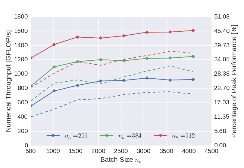
Figure 3: Numerical throughput achieved with the CUDA GPU backend using two compute streams (solid) compared to the standard implementation (dashed).
Double Precision
Since the implementation is generic with respect to the floating point type used in the calculations, the same benchmarks have been performed once again using double precision arithmetic. The use of double arithmetic of course reduces the numerical throughput, relative to the peak performance of the device, however, the numerical throughput is actually improved.
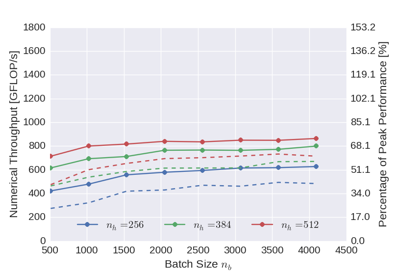
Figure 4: Numerical throughput achieved with the CUDA GPU backend using double precision arithmetic. Solid lines display the performance achieved using two compute streams, while the dashed lines one show the performance achieved using only one compute stream.
Profiling Results
In addition to the overall numerical throughput, also execution profiles were recorded for the CUDA implementation. The fractions of the execution time spent in the different computational routines of the low-level interface are given in the figure below. As predicted by the performance, most of the compute time is consumed by matrix multiplications (GEMM), followed by the application of the activation functions and their derivatives.
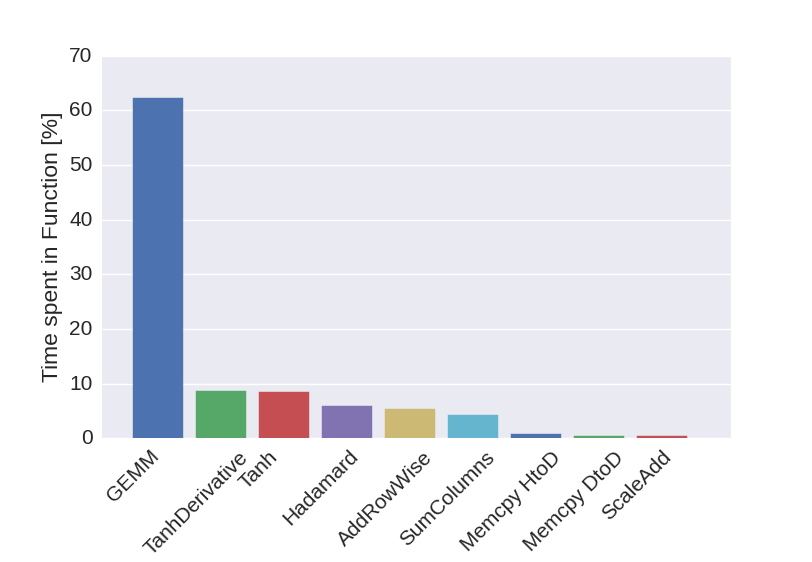
Figure 5: Fraction of the compute time spent in the different sub-routines of the low-level interface.
OpenCL Backend
Finally, also an OpenCL backend for the deep neural network implementation has been developed. This has not yet been integrated into Root master in order to test on additional architectures prior to releasing it. The numerical throughput achieved on the Nvidia Tesla K20 card is displayed in the plot below. The performance is clearly inferior compared to the CUDA implementation, which was somehow expected considering that OpenCL supports a large range of compute architectures.
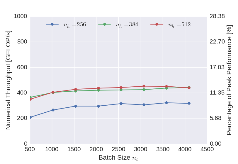
Figure 6: Computational performance of the OpenCL backend.
Summary
In this post the performance results obtained for the different backends have been presented. Compared to the CPU implementation, the CUDA implementation performs significantly better. Unfortunately we were not able to achieve the same performance with the OpenCL implementation. The performance results are summarized in the bar plot below, comparing the performance achieved for a batch size \(n_b = 1024\). The plot also shows the performance that was obtained using the Lasagne python package, which uses Theano for GPU-accelerated matrix arithmetic. The Lasagne-benchmark was also performed on the Nvidia Tesla K20.
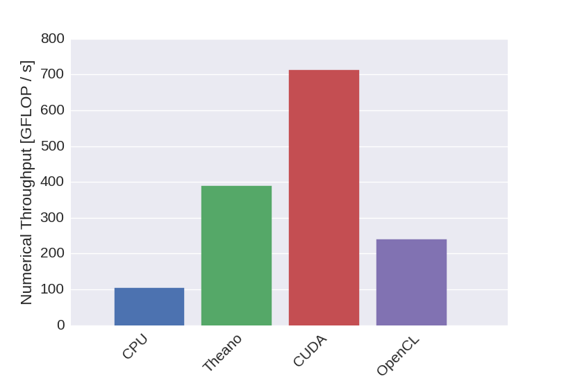
Figure 7: Numerical throughput achieved with the newly developed neural network implementation.