Training Deep Neural Networks on GPUs
After the successful integration of the deep neural network prototype into TMVA described in the last post, the next milestone was the development of a GPU backend for the neural network implementation. While the implementation itself was ready relatively quickly, it took until now to get the code ready for integration into the TMVA master branch and test the implementation on the Higgs benchmark dataset.
The CUDA DNN Backend
This first implementation of a GPU backend for deep neural networks was developed using NVIDIAs CUDA API. While it is also planned to develop an OpenCL backend for the deep neural network implementation in TMVA, the choice to start with a CUDA implementation was mainly based on me being more familiar with the CUDA API as well as the improved (expected) performance on CUDA devices.
The implementation uses cuBLAS for the linear algebra function required in the backend including matrix-matrix multiplication (cublasDgemm) and scaled matrix addition (cublasDaxpy). For the application of activation functions, computation of their gradients, evaluation of loss and regularization functionals as well as application of dropout, the implementation uses its own kernels in order to minimize external dependencies.
Data Transfer
Excessive data transfers are the weak spot of GPGPU programming. GPU computing architectures generally dispose of only a limited amount of directly accessible device memory and transferring data from the host is expensive. While the training of deep neural networks may require the transfer of large amounts of training data to the GPU, the transfers are independent from the actual computation and the training data can therefore easily be preloaded and transfers overlapped with computation.
The approach taken here is to continuously stream the data instead of moving all training data to the device at the beginning of the training. This will allow for greater flexibility when running on devices with limited memory or training on very large data sets. The streaming is handled by an architecture specific data loader class. This data loader class provides begin() and end() methods that allow the user to iterate over the batches in a training epoch. Each batch object in turn provides access to the training data through GetInput() and GetOutput() member functions, which return a batch of training data in matrix representation. The class structure of the generic training class and the CUDA backend class is illustrated in the figure below.
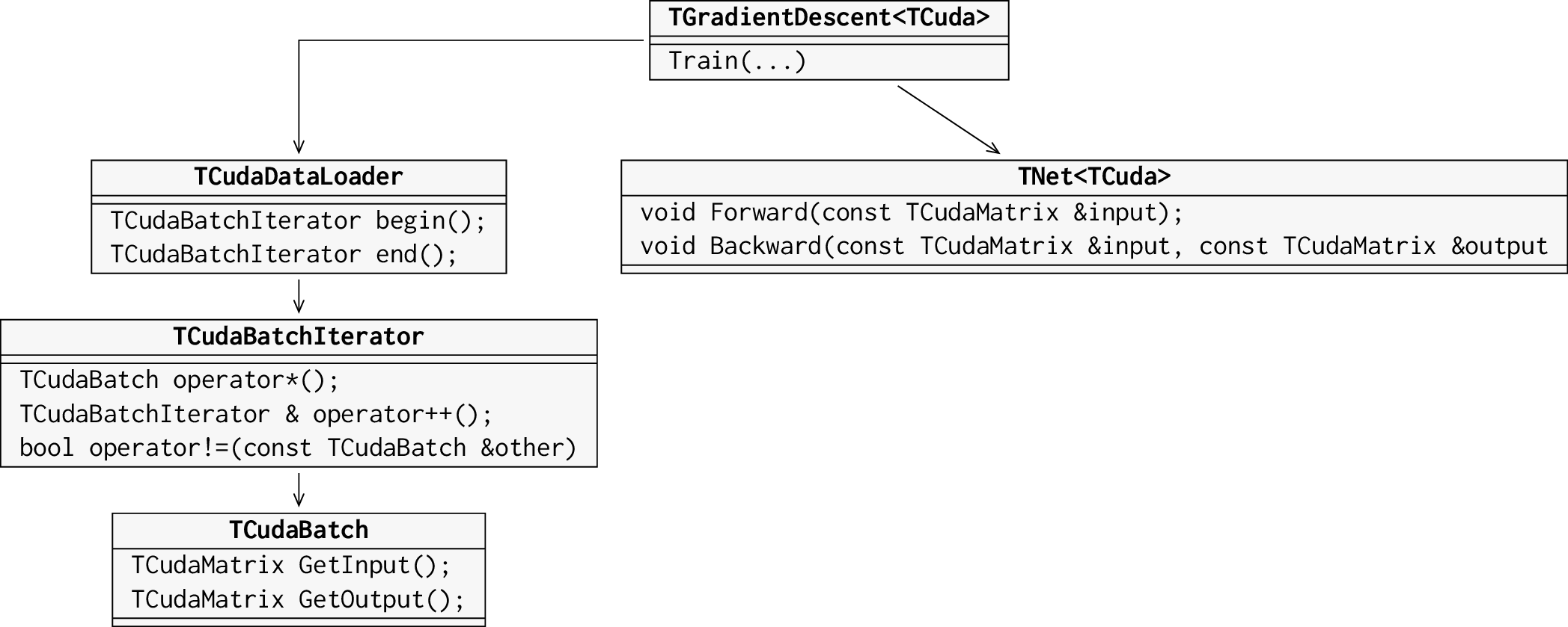
Figure 2: Cuda implementation of the data streaming interface for the training of deep neural networks.
Benchmark Tests
In order ensure correctness of the GPU implementation as well as to get a first impression of its computational performance, the CUDA backend was used to train a neural network on the Higgs dataset and its classification performance compared to the original CPU deep neural network implementation.
I encountered some problems with the original implementation of neural networks in TMVA, the one used in my first post, which forced me to keep the network relatively small. The network structure is given in the table below:
| Number of Neurons | Activation Function | |
|---|---|---|
| Input Layer | 28 | Identity |
| Hidden Layer 1 | 100 | \(\tanh\) |
| Hidden Layer 2 | 50 | \(\tanh\) |
| Hidden Layer 3 | 10 | \(\tanh\) |
| Output Layer | 1 | Sigmoid |
Both implementations were trained using cross entropy loss and a learning rate of \(0.02\). No regularization such as weight decay or dropout has been applied. During preprocessing, a Gaussian transformation has been applied to the input data, which transformed the input features so that their distributions ressemble Gaussian distributions.
In total three different tests were performed with increasing training set sizes. The first test started out with \(5 \times 10^5\) training samples, the second one used \(10 ^6\) and the third one \(2 \times 10^6\).
Classification Performance
As primary performance measure the area under the ROC curve of the classifier is used. The results are given in Table 2 below. As expected, the performance increases with the size of the training set. However, the old implementation does not achieve the same classification performance as the GPU implementation. While it is difficult to pinpoint the exact cause of the underperformance of the CPU implementation, it is likely attributable to differences in the training implementation.
| No. of Training Samples | Area Under ROC Curve - CPU | AreaUnder ROC Curve - GPU |
|---|---|---|
| \(5 \times 10^5\) | 0.824 | 0.82 |
| \(1 \times 10^6\) | 0.841 | 0.826 |
| \(2 \times 10^6\) | 0.846 | 0.831 |
Computational Performance
The overall computational performance of the two implementations is given by the total training time together with the number of training epochs that were performed. The CPU version was running in parallel on a 32-core Intel Xeon E5 2650 while the GPU implementation was running on a NVIDIA Tesla K20. Looking at the results given in Table 3, one can clearly see that the CPU version outperforms the GPU version with respect to number of training epochs per unit time. This, however, is not very suprising considering that the CPU version is parallelized using Hogwild! style, which means that training on different batches is performed in parallel. Given the size of the training set, the CPU implementation can thus fully exploit the performance of the 32 cores. On the GPU the batches are processed sequentially, but the processing of each batch is parallelized. For small batch sizes, this obviously makes exploiting the full computing power of the GPU difficult.
| No. of Training Samples | Time CPU [s] | Epochs CPU | Time GPU [s] | Epochs GPU |
|---|---|---|---|---|
| \(5 \times 10^5\) | \(714\) | 160 | \(1280\) | 189 |
| \(1 \times 10^6\) | \(2280\) | 295 | \(3260\) | 224 |
| \(2 \times 10^6\) | \(4470\) | 288 | \(8103\) | 182 |
Summary and Outlook
The benchmark tests described above mark the first real-world application of the GPU-accelerated implementation of deep neural networks that has been developed in the course of this GSoC project and thus constitute another important step towards multi-architecture, accelerated training of deep neural networks in TMVA.
While the computational performance of the training still leaves room for improvements, the classification performance of the GPU implementation looks promising. The next steps for the GPU implementation are thus an in-depth performance analysis in order to better exploit the computational performance of the device as well as improving the classification performance on the Higgs dataset by refining the network structure and training process.
In parallel to this, also the development of an optimized CPU implementation that fixes the shortcomings of the old implementation as well as an OpenCL backend for the neural network implementation has been started.