In my last blog post, I presented a first prototype of a multi-architecture implementation of deep feedforward neural networks. While the different components of the prototype were thoroughly tested using unit tests, the next step was to integrate the prototype into TMVA in order to perform an end-to-end test of the system, which compares the classification performance of the prototype to the performance of the original implementation of deep neural networks in TMVA.

Neural Network Training

So far I have not discussed how the training of the neural network prototype will be performed. In general, neural networks are trained iteratively using gradient-based optimization methods. This means in each step the weights \(\mathbf{W}^l\) and bias terms \(\boldsymbol{\theta}^l\) of each layer \(l\) are updated based on the gradients of the loss function with respect to the weights and bias terms:

In general, the weight and bias-term updates, \(\Delta \mathbf{W}^l\) and \(\Delta\boldsymbol{\theta}^l\) may depend also on the previous minimization steps that have been performed. For now, however, we will only consider the simplest gradient-based minimization method, namely gradient descent, where the weight updates in each step are given by

for a given learning rate \(\alpha\). Using the scale_add function defined in the low-level interface, a gradient descent step for a given mini-batch from the trainin set can be implemented by performing forward and backward propagation and adding the computed weights and bias gradients to the weights and biases of each layer.

net.Forward(input);
net.Backward(input, output);

for (size_t i = 0; i < net.GetDepth(); i++)
{
    auto &layer = net.GetLayer(i);
    scale_add(layer.GetWeights(), layer.GetWeightGradients(),
                1.0, -fLearningRate);
    scale_add(layer.GetBiases(), layer.GetBiasGradients(),
                1.0, -fLearningRate);
}

Note that input and output are the input events and true labels of a mini batch from the training set in matrix form. The mini batches are generated by shuffling the training set and splitting it up into of a given batch size. Then, a single minimization step is performed on each of the batches. The number of minimization steps required to traverse the complete training set is called an epoch. Convergence of the algorithm is determined by periodically monitoring the loss or error on a validation set. Convergence is assumed to be achieved when the minimum loss on the validation set has not decreased for a given number of epochs.

The integration of the prototype into TMVA took me the last two weeks. The reason for the delay is that I decided to also refactor the implementation of the TMVA interface after discovering some bugs and shortcomings in the original implementation of DNNs in TMVA.

Results

For the testing, a subset of the higgs data set described in my first blog post was used. The data set consists of 9000 background and 9000 signal training events as well 1000 test events of each class. The training was performed using a very simple neural net consisting of 3 hiden layers with 100, 50 and 10 neurons with ReLU activation functions for the first two hidden layers and identity activations on the last one. The relevant TMVA configuration settings are given below:

TString configString = "!H:V";
configString += ":VarTransform=G";
configString += ":ErrorStrategy=CROSSENTROPY";
configString += ":WeightInitialization=XAVIERUNIFORM";
TString layoutString = "Layout=RELU|100,RELU|50,RELU|10,LINEAR";
TString trainingString = "TrainingStrategy="
                         "LearningRate=0.0005,"
                         "Momentum=0.0,"
                         "Repetitions=1,"
                         "ConvergenceSteps=10,"
                         "BatchSize=20,"
                         "Regularization=None,"
                         "TestRepetitions=15,"
                         "Multithreading=False";

configString += ":" + layoutString + ":" + trainingString;
TMVA::Types::EMVA method = TMVA::Types::kDNN;
factory->BookMethod(loader, method, "DNN", configString);

The rootbook used for the tests can be found here. The training was performed using standard gradient descent with a learning rate of \(\alpha = 5 \times 10^{-4}\) and 10 steps without improvement in the minimum network loss required for convergence (ConvergenceSteps). The trained networks are evaluated by computing the ROC curve of the corresponding classifier. The results are displayed in the figure below. The black line displays the result from the prototype and the red line the result from the original implementation. As can be seen from the plot, both methods achieve nearly identical classification performance.

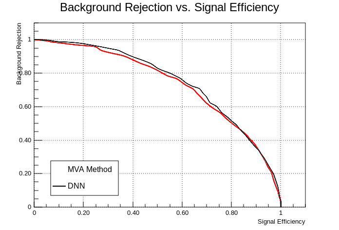
Figure 1: ROC curve of the deep neural network prototype trained on a subset of the Higgs dataset (black). The red curve displayes the performance of the original implementation.

The time required for the training of the neural networks were \(231 s\) and \(317 s\) for the new prototype and the previous implementation, respectively. While I do not expect the reference implementation to be numerically more efficient than the previous implementation, the reduction in training time may be due differences in the implementation of the networks. The previous implementation includes a bias term only for the first layer, while the current implementation uses them on every layer. This may provide additional flexibility which allows the net to adapt to the training set in less training steps. However, this is just a suspicion and a more detailed analysis will be required to make any knowledgable statements about the performance of the two implementations.

Summary and Outlook

With the successful integration of the neural network prototype into TMVA, an important milestone on the way towards GPU-accelerated training of neural networks in TMVA was achieved. The prototype currently implements the core functionality required to train and evaluate the neural network. Moreover, the reference implementation and the generic unit tests developed so far should considerably simplify the implementation of hardware-specific backends. The next step from here will be to implement a first GPU backend in order demonstrate the capabilities of the current design.